Deep Learning with Pytorch by NYU (part 1)

1. TL;DR: What happened?

Here’s a set of condensed notes for the NYU course about pytorch. Instead of simply taking full notes, which I’m sure someone before me has done a better, job, I’ll try to focus on resources I used, as well as useful informations given orally, which I did not hear elsewhere.

Please

2. Resources

• Companion website for the pytorch course offered by NYU.
• PyTorch fundamentals overview
• Good Introduction to Computational Graphs

3. W1: Introduction

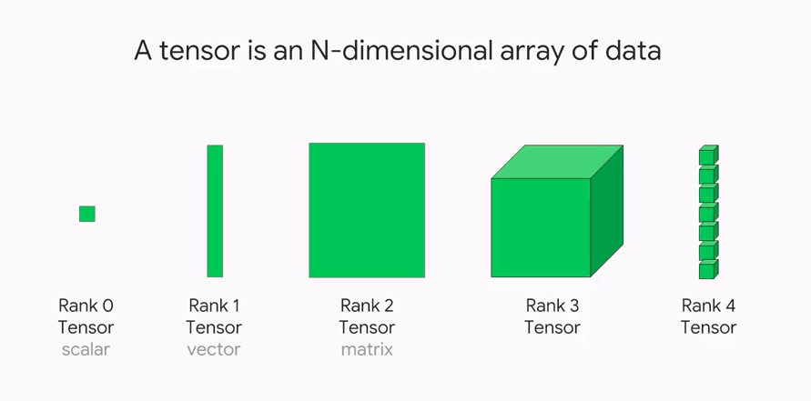
Tensors

source

4. Stochastic Gradient Descent

Example of Gradient Descent with Quadratic Function

Suppose we have an unknown quadratic function for which we would like to estimate the parameters.

time = torch.arange(0,20).float(); time
# This is the function we wish to estimate.
# We do NOT know the actual values of the parameters.
speed = torch.randn(20)*3 + 0.75*(time-9.5)**2 + 1

We know that the function must be in the form a*(time**2)+(b*time)+c, so it’s a matter of estimating a, b, and c and making them as close to the “true” a, b, and c as possible.

First, we set up a helper function for outputting a value given a set of estimated coefficients a' b' c' under the premise that the true function form is quadratic.

def func(t, params):
    a,b,c = params
    return a*(t**2) + (b*t) + c

Then, we choose a loss function for assessing the quality of a given set of coefficients. In this case, we use the mean squared error (MSE)

def mse(preds, targets): return ((preds-targets)**2).mean().sqrt()

Now, we begin a 7 step process of improving our estimate.

1. Initialize the parameters a' b' and c'

# Here we initialize a tensor [a, b, c] of rank 1 holding 3 random numbers, and tag them with the _requires_grad_()
params = torch.randn(3).requires_grad_()

2. Compute the initial prediction using func(time, params).
3. Compute loss for our initial prediction using loss = mse(preds, speed). (Note: this loss function may be different depending on the problem you’re working with!)
4. Compute the gradient using loss.backward(). (**Note when you call backward(), the previous computional graph is thrown away!)
5. “Step” the weights in the right directions and reset the gradient values. lr is the learning rate, an arbitrarily small number.

   lr = 1e-5
   params.data -= lr * params.grad.data
   params.grad = None

6. Reiterate an arbitrary amount of time.

Put together, it becomes the following:

# Define the "truth". In a training dataset, this would be the labeled data. 
speed = torch.randn(20)*3 + 0.75*(time-9.5)**2 + 1

# Definition of evaluation function
def f(t, params):
    a,b,c = params
    return a*(t**2) + (b*t) + c

# Definition of loss computation
def mse(preds, targets): return ((preds-targets)**2).mean().sqrt()

# Step 1. Random initialization of parameters 
params = torch.randn(3).requires_grad_()
# Step 2. Compute initial prediction
preds = f(time, params)
# Step 3. Compute loss from initial prediction and truth
loss = mse(preds, speed)